Arithmetic Mean
The arithmetic mean, often denoted as μ or x̅, for a dataset of n observations x1,x2,…,xn is defined as:

We want to find a recurrence relation that allows us to update the mean x̅n to x̅(n+1) when a new data point x(n+1) arrives, without re-summing all previous data points.
Consider the mean after n+1 observations:

We can separate the sum:

We know that:

Substituting this into the equation:
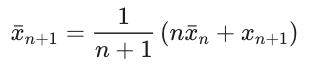
Now, let’s manipulate this to show the incremental update:

We can rewrite

The final steps

This is the recurrence relation for the arithmetic mean. It shows that the new mean is the old mean plus a fraction of the difference between the new data point and the old mean.
Variance
The sample variance, often denoted as s2 or σ2, for a dataset of n observations x1,x2,…,xn is defined as:

For an online algorithm, it’s often more convenient to work with the sum of squares of differences from the mean, also known as the sum of squared errors (SSE) or M2:


We know that:

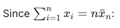

Now, consider M2,n+1 when a new data point xn+1 arrives:

We can use the property that for any value c:

If we put c = x̅:

Using the property on the first term:

So, we have:

We know the recurrence for the mean:

From this, we can derive:

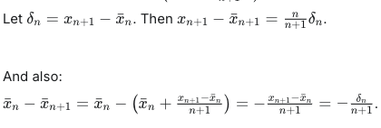
Substituting these into the equation for M2,n+1:

This is the recurrence relation for the sum of squared differences M2.
Now, for the variance itself:
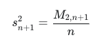
For n>1:
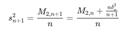
This can be written as:
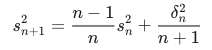
Where δn=xn+1−x̅n. This is a robust online formula for variance (often referred to as Welford’s algorithm or a variant of it).
JavaScript Implementation of Online Algorithms
let current_n = 0;
let current_mean = 0;
let current_sum_sq_diff = 0;

function addValue(newValue) {
    current_n++;
    if (current_n === 1) {
        current_mean = newValue;
        current_sum_sq_diff = 0;
    } else {
        const oldMean = current_mean;
        current_mean = oldMean + (newValue - oldMean) / current_n;
        current_sum_sq_diff += (newValue - oldMean) * (newValue -current_mean);
    }

function resetStatistics() {
    current_n = 0;
    current_mean = 0;
    current_sum_sq_diff = 0;
}

function getCount() {
    return current_n;
}

function getMean() {
    return current_mean;
}

function getSampleVariance() {
    if (current_n < 2) {
        return 0;
    }
    return current_sum_sq_diff / (current_n - 1);
}

function getPopulationVariance() {
    if (current_n === 0) {
        return 0;
    }
    return current_sum_sq_diff / current_n;
}

function getSampleStandardDeviation() {
    return Math.sqrt(getSampleVariance());
}

function getPopulationStandardDeviation() {
    return Math.sqrt(getPopulationVariance());
}
Discussion on Advantages of Online Algorithms
Numerical Stability
- Error Propagation: Batch algorithms often calculate the sum of squares (
∑xi2) and the sum ofxi(∑xi) separately and then combine them (e.g.,Var=n∑xi2−(n∑xi)2). Whenxivalues are large but their variance is small (i.e., data points are close together but large in magnitude),∑xi2and(∑xi)2/ncan be very large numbers that are nearly equal. Their subtraction can lead to a loss of significant digits due to catastrophic cancellation. - Welford’s Algorithm (for Variance): Online algorithms, especially Welford’s method for variance, are designed to mitigate this. They compute the sum of squared differences from the current mean (
M2) incrementally. The difference delta = newValue – this.mean is typically a much smaller number than the raw values themselves, or their squares, reducing the magnitude of numbers being added or subtracted. This keeps the intermediate calculations within a more stable range for floating-point arithmetic. The delta * delta2 term ((newValue – oldMean) * (newValue – newMean)) ensures that we are always dealing with differences, which are less prone to large cumulative errors.
Error Propagation
Online algorithms minimize error propagation because each step is an incremental adjustment based on the new data point and the currently accumulated statistics. In batch methods, small errors in individual sums (∑xi or ∑xi2) can accumulate and be magnified when combined in the final calculation, especially during subtraction of large, nearly equal numbers. Online algorithms, by focusing on differences from the mean, effectively “re-center” the calculations with each new data point, preventing the accumulation of large absolute errors that can occur when dealing with large raw numbers.
Catastrophic Cancellation
As mentioned under numerical stability, catastrophic cancellation is a primary concern with batch variance calculation. Consider a dataset like [10^9, 10^9 + 1, 10^9 + 2].
Batch approach:

This involves subtracting two very large numbers (3×10^18 and a number very close to it). If using standard floating-point numbers (e.g., IEEE 754 double-precision), the result can lose all precision and become inaccurate or even zero due to the limited number of significant digits.
Online approach (Welford’s):
- The delta terms (e.g., newValue – mean) are small values like 1, 0, -1.
- The M2 (sum of squared differences) accumulates these small differences directly.
- This avoids the subtraction of large, nearly equal numbers entirely, making it highly robust against catastrophic cancellation.
Overflow Management
Batch algorithms calculating ∑(xi)^2 can lead to overflow if xi are large, even if the final variance is small. For example, if xi=10^10, then (xi)^2=10^20. A sum of many such (xi)^2 values can easily exceed the maximum representable number for standard floating-point types.
Online algorithms like Welford’s primarily operate on differences from the mean. While the mean can still grow large, the delta values remain relatively small if the new data points are close to the current mean. The M2 term, which tracks the sum of squared differences, is much less likely to overflow because it sums smaller numbers. This greatly reduces the risk of overflow compared to summing raw squared values.
Computational Efficiency
- Time Complexity: Both batch and online algorithms typically have a time complexity of
O(N), whereNis the number of data points. Each data point in an online algorithm requires a constant number of arithmetic operations (addition, subtraction, division). A batch algorithm also iterates through the data once (or twice, if calculating∑xiand∑(xi)^2in separate passes). So, from an asymptotic perspective, they are similar. However, online algorithms perform calculations incrementally, which can be more efficient in streaming data scenarios where data isn’t available all at once. - Memory Efficiency: This is a major advantage of online algorithms. They only need to store a few variables (count, mean, M2) regardless of the number of data points. They do not need to store all the raw data points in memory. Batch algorithms, especially those that need to make multiple passes or store the entire dataset, can be very memory-intensive, requiring
O(N)memory. This makes online algorithms ideal for processing very large datasets or data streams where storing everything is infeasible.
Robustness and Scalability
- Robustness: Online algorithms are inherently more robust to outliers and noisy data. While a single outlier can significantly shift the mean and variance, the online method processes it one step at a time, providing a continuous update. Their numerical stability also contributes to their robustness against floating-point inaccuracies.
- Scalability: Due to their constant memory footprint and
O(1)computation per new data point, online algorithms are highly scalable. They can handle datasets of virtually any size, from a few points to billions, without running out of memory or experiencing a significant degradation in performance per update. This makes them indispensable in big data analytics, real-time monitoring, and embedded systems where resources are limited.