Concepts of location and dispersion measures

In statistical analysis, a central objective is to transform complex and extensive datasets into concise and interpretable summaries. When dealing with hundreds or thousands of observations, reporting each individual data point is not only impractical but also risks obscuring the underlying structure and meaningful patterns within the dataset. Consequently, measures of central tendency and location constitute indispensable analytical tools.

These measures enable researchers to identify the “center” of a distribution and to characterize its typical or representative value through a single summary statistic. Nonetheless, the heterogeneous nature of real-world data necessitates a nuanced approach. Data distributions may be symmetric or skewed, influenced by extreme values, composed of proportions or rates, or even classified into categorical groups. As a result, no single measure is universally appropriate across all contexts.

The arithmetic mean, median, and mode—as well as more specialized measures such as the geometric and harmonic mean—respond differently to distributional features and serve distinct analytical purposes. Therefore, selecting the most suitable measure requires careful consideration of the data type, the presence of outliers, and the specific aspect of the distribution that one intends to capture or emphasize.

The Concept of Central Tendency

To illustrate with a practical example: when comparing the performance of two products using customer ratings, simply presenting each individual rating in a table offers minimal analytical value. What is needed instead is a single summary statistic that encapsulates the aggregate satisfaction level. This representative value is termed a measure of central tendency.

Measures of central tendency summarize a dataset by identifying a central or typical value around which the data points tend to cluster. The three most common measures are:

• Mean (arithmetic average): is calculated by adding all the values in a dataset and dividing by the number of observations. It represents the typical value, but it can be strongly affected by very high or very low values (outliers).
• Median (middle value): the middle value when all observations are ordered from smallest to largest. If the dataset has an even number of values, it is the average of the two middle numbers. It is useful because it is not influenced by outliers and better represents the “central” value in skewed distributions.
• Mode (most frequent value): is the value that appears most frequently in a dataset. A dataset can have one mode, more than one mode, or none at all (if no value repeats). It is especially useful for categorical data or when identifying the most common value is important.

Each of these measures highlights a different aspect of the data and is appropriate under different circumstances.

The Arithmetic Mean

Definition

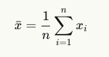
The arithmetic mean, commonly referred to as the “average,” is calculated by summing all values in a dataset and dividing by the number of observations:

When to Use

The mean is ideal when:

• Data is approximately symmetric and follows a normal distribution
• You want a measure that incorporates every observation in the dataset
• Extreme values are representative of the underlying process, not anomalies

Advantages: 

Its biggest strength is that it uses every single piece of data you have. Every height, every age, every score contributes to its calculation. This makes it very useful when you want a measure that reflects the entire distribution of your data, and it has excellent mathematical properties that make it a solid foundation for more complex statistical analyses. Plus, for any given set of numbers, there’s always only one mean.

Limitations

The mean is highly sensitive to outliers. A single extreme value can disproportionately shift the mean away from the typical range of the data. For instance, in income data, a few extremely high salaries can inflate the mean, making it unrepresentative of the typical household income.

Example

Consider exam scores: {65, 70, 72, 75, 78, 80, 82}. The mean is 74.6, which accurately represents the center of this symmetric distribution. However, if one score is 100 instead of 82, the mean jumps to 77.1, even though most students scored in the low-to-mid 70s.

The Median

Definition

The median is the middle value when data is arranged in ascending order. For datasets with an odd number of observations, it’s the central value; for even-numbered datasets, it’s the average of the two central values.

When to Use

The median is preferred when:

• Data is skewed or contains outliers
• You need a measure that represents the “typical” observation without being influenced by extremes
• Working with ordinal data (ranked categories)

Advantages

The median is robust to outliers because it’s the position, not the magnitude of the value, that matters. This makes it particularly valuable in fields like real estate (housing prices), income analysis, and any domain where outliers are common but not representative. So, it is an excellent measure for datasets with outliers or strong skewness (like incomes or house prices), where a few very high values could distort the mean.

Limitations

Because it only looks at the central position, the median ignores most of the information contained in the other data points. It doesn’t consider how big or small the other numbers are, only where they fall in relation to the center. To calculate it, you must first sort all the data, which can be computationally intensive for very large datasets. It also has fewer mathematical properties than the mean, making it less versatile for advanced statistical analysis.

Examples

Example with odd number of dataset: In the dataset {20, 25, 30, 35, 200}, the mean is 62, which is misleading since most values cluster around 25-35. The median is 30, which better represents the typical value.

The Mode

Definition

The mode is the value that appears most frequently in a dataset. A dataset can be:

• Unimodal (one mode)
• Bimodal (two modes)
• Multimodal (multiple modes)
• No mode (all values occur with equal frequency): Each number appears only once. So, there is no mode for this dataset.

When to Use

The mode is especially useful for:

• Categorical data where mean and median are not applicable (e.g., favorite color, brand preference)
• Discrete data (e.g., number of children per family)
• Identifying the most common or popular value

Advantages

Its biggest advantage is that it can be used with any type of data, including categorical (nominal) data (like favorite colors or car brands), which the mean and median cannot do. It’s completely unaffected by outliers because it focuses solely on frequency. It immediately tells you what the most popular or common item/category is, which is useful in many practical contexts.

Limitations

The mode can be a bit tricky. You might have a dataset with no mode at all (if all values appear the same number of times), or you might have multiple modes (bimodal, multimodal), which can make it harder to define what’s “typical.” Like the median, the mode also disregards most of the information in the dataset, focusing only on what’s most frequent. Sometimes, a value that appears only slightly more often than others might be the mode but doesn’t truly represent the “center” or the majority of the data. Its mathematical properties are very limited, making it less useful for in-depth quantitative analysis.

Example

Unimodal: In shoe size data {7, 8, 8, 8, 9, 10, 11}, the mode is 8—the most commonly purchased size, which is valuable information for inventory management.

Multimodal: In shoe size data {7, 8, 8, 9, 9, 10, 10, 11}, the modes are 8, 9, 10— they appear most frequently.

Different types of Mean

Weighted Average

The Weighted Average is a type of arithmetic mean where some data points contribute more than others to the final average. Instead of each value having an equal say, certain values are given a “weight” that reflects their importance or frequency. If you have a set of values x1​,x2​,…,xn​ and corresponding weights w1,w2,…,wn​, the weighted average is calculated as:

Relationship with Arithmetic Mean

The arithmetic mean is actually a special case of the weighted average! If all the weights are equal (or if all weights are 1), the weighted average simplifies to the standard arithmetic mean. For example, if you have exam scores where the final exam counts more than a quiz, you’d use a weighted average. If all assignments counted equally, it would just be an arithmetic mean.

Geometric Mean

The Geometric Mean is a type of average that is most appropriate for sets of positive numbers that are linked or multiplied together, such as rates of growth, percentages, or ratios. It’s particularly useful when dealing with data that grows exponentially or when calculating the average of ratios. For a set of n positive numbers x1​,x2​,…,xn​, the geometric mean (GM) is calculated by multiplying all the numbers together and then taking the n-th root of the product:

Relationship with Arithmetic Mean

The geometric mean is always less than or equal to the arithmetic mean for any set of positive numbers (unless all the numbers are identical, in which case they are equal). This is a significant mathematical property known as the AM-GM inequality. It tends to “dampen” the effect of very large values and is less sensitive to outliers than the arithmetic mean when dealing with percentage changes or growth rates. If you were averaging returns on an investment over several years, the geometric mean would give you the true average annual growth rate, which the arithmetic mean would typically overestimate.

Harmonic Mean

The Harmonic Mean is particularly useful for averaging rates or ratios when the values are expressed as units per time (or vice versa), and when the total “effort” or “task” is consistent across the different rates. Common applications include averaging speeds over fixed distances, or averaging performance rates. For a set of n positive numbers x1​,x2​,…,xn​, the harmonic mean (HM) is calculated as the reciprocal of the arithmetic mean of the reciprocals of the numbers:

Relationship with Arithmetic Mean

For any set of positive numbers, the harmonic mean is always less than or equal to the geometric mean, which in turn is less than or equal to the arithmetic mean (HM ≤ GM ≤ AM). This relationship, along with AM-GM, forms the AM-GM-HM inequality. The harmonic mean is heavily influenced by the smallest values in the dataset and is less affected by large outliers than the arithmetic mean. For instance, if you’re averaging speeds for a round trip where the distance is fixed, the harmonic mean gives the correct average speed, whereas the arithmetic mean would often be misleading.

Quadratic Mean (Root Mean Square – RMS)

The Quadratic Mean, also widely known as the Root Mean Square (RMS), is most often used when dealing with quantities that vary over positive and negative ranges, and where the magnitude of the values is more important than their direction. It’s particularly common in physics and engineering, for example, to calculate the average magnitude of alternating current (AC) or voltage, or the speed of gas molecules. It effectively gives a measure of the typical magnitude of a set of numbers, especially when some are negative. For a set of n numbers x1​,x2​,…,xn​ the quadratic mean (QM or RMS) is calculated by taking the square root of the arithmetic mean of the squares of the numbers:

Relationship with Arithmetic Mean

For a set of numbers, the quadratic mean is always greater than or equal to the arithmetic mean (QM ≥ AM), unless all numbers are zero or the same, in which case they are equal. The key difference is that by squaring the values, RMS emphasizes larger values more than the arithmetic mean does, and it handles negative values by turning them positive before averaging. This means it measures the “effective” or “typical” magnitude of the numbers, often when they represent fluctuating quantities. It effectively penalizes larger deviations more heavily than the arithmetic mean would.

Measures of Dispersion

Range

The Range is the most straightforward measure of dispersion, defined as the difference between the maximum and minimum observed values in a dataset. Given a dataset X={x1​,x2​,…,xn​}, the Range (R) is calculated as: R=max(X)−min(X)

Properties:

• Simplicity: It is exceptionally easy to compute and interpret.
• Sensitivity to Extremes: The Range is highly susceptible to the influence of outliers, as it is determined solely by the two most extreme values in the dataset. Consequently, it may not be representative of the typical spread of the data, especially in the presence of anomalies.
• Information Loss: It provides no information about the distribution of data points between the minimum and maximum values.

The Range is generally suitable for preliminary data exploration or for small datasets where a quick, approximate measure of spread is sufficient. Its utility diminishes in larger, more complex datasets or those prone to extreme values.

Variance

Variance is a foundational measure of dispersion that quantifies the average squared deviation of each data point from the mean of the dataset. It provides a comprehensive measure of the overall spread of data by accounting for every observation.

For a population of N data points {x1​,x2​,…,xN​} with a mean μ, the population variance (σ^2) is defined as:

For a sample of n data points {x1​,x2​,…,xn​} with a sample mean x̅, the sample variance (s^2) is defined as:

The use of n−1 in the denominator (Bessel’s correction) provides an unbiased estimator of the population variance when calculated from a sample.

Properties:

• Comprehensive: It incorporates all data points in its calculation, offering a more robust measure of variability than the Range.
• Units: The units of variance are the square of the original data units, which can impede intuitive interpretation in practical contexts. For instance, if data are measured in kilograms, variance is expressed in square kilograms.
• Mathematical Tractability: Its mathematical properties make it amenable to various statistical theories and inferential procedures.

Variance is a crucial component in many statistical models, including regression analysis, and hypothesis testing. While its direct interpretability is limited due to squared units, its theoretical importance is paramount.

Standard Deviation

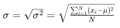
The Standard Deviation is the most widely adopted measure of dispersion, representing the square root of the variance. By reverting the units to those of the original data, it offers a more interpretable and practical measure of the typical deviation of data points from the mean.

For a population, the standard deviation (σ) is:

For a sample, the standard deviation (s) is:

Properties:

• Interpretability: Expressed in the same units as the original data, facilitating direct interpretation (e.g., a standard deviation of 5 kg indicates a typical deviation of 5 kg from the mean weight).
• Sensitivity to Outliers: While more robust than the Range, it is still influenced by extreme values, although to a lesser extent than the Variance due to the square root operation.
• Empirical Rule: For normally distributed data, approximately 68% of data falls within one standard deviation of the mean, 95% within two, and 99.7% within three.

Standard deviation is extensively used across virtually all quantitative disciplines for describing data variability, comparing distributions, constructing confidence intervals, and performing hypothesis tests. It is particularly valuable when data are approximately symmetrically distributed.

Interquartile Range (IQR)

The Interquartile Range (IQR) is a robust measure of dispersion that describes the spread of the central 50% of the data. It is particularly useful for datasets that are skewed or contain outliers, as it is less sensitive to extreme values compared to the Range or Standard Deviation. To calculate the IQR, the data must first be ordered. The quartiles are defined as follows:

• First Quartile (Q1): The value below which 25% of the data fall. It is the median of the lower half of the dataset.
• Third Quartile (Q3): The value below which 75% of the data fall. It is the median of the upper half of the dataset.

The IQR is then calculated as the difference between the third and first quartiles: IQR=Q3−Q1

Properties:

• Robustness to Outliers: Since the IQR focuses on the central portion of the data, it is highly resistant to the influence of extreme values, making it an appropriate measure for skewed distributions.
• Non-parametric: It does not assume any particular distribution shape for the data.
• Complementary to Median: The IQR is often reported alongside the median, providing a comprehensive summary of the central tendency and spread for non-normal or ordinal data.
• Outlier Detection: IQR is also used to identify potential outliers, where values falling below Q1−1.5×IQR or above Q3+1.5×IQR are considered outliers.

IQR is indispensable in exploratory data analysis, particularly when visualizing data with box plots. It is preferred for financial data, income distributions, and other datasets where outliers are common and the distribution is not Gaussian.