This report discusses the analogies between the server security simulation (HMWK 7) and a classic Bernoulli process simulation of the Law of Large Numbers (LLN). It highlights the key similarities and differences by referencing the results of the first assignment. Furthermore, it illustrates the deep-rooted mathematical properties connecting the simulation to binomial coefficients, Pascal’s triangle, binomial expansion, and the Fibonacci sequence.
Analogies with the Bernoulli Process and the Law of Large Numbers
At the core of the server security simulation lies the Bernoulli process, a sequence of n independent and identically distributed (i.i.d.) random experiments, where each trial can result in one of two outcomes: “success” or “failure.” In this context:
- Trial: A single week of server operation.
- Success: The server remains secure (score of +1), occurring with probability
1−p. - Failure: The server is breached (score of -1), occurring with probability
p.
Although this framework is common to many probabilistic models, the analytical objective determines the theoretical perspective to be adopted.
Both the random walk model and simulations designed to illustrate the Law of Large Numbers (LLN) share the same underlying stochastic architecture. They are both based on the summation or averaging of i.i.d. Bernoulli random variables. This common foundation is why their mathematical properties are so closely intertwined.
Explicit connection with the Law of Large Numbers
The empirical average of Bernoulli outcomes satisfies
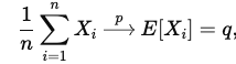
where q=(1-p)^m is the probability that the server remains secure in a given week.
For the cumulative score

this implies
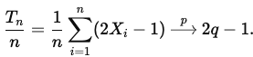
Hence, the random walk converges in probability to its drift 2q−1, showing that the long-term average behaviour of the cumulative score is governed by the same LLN that controls the frequency of secure weeks.
The crucial difference lies in the object of investigation
- Objective of the Random Walk (HMWK 7): Analysis of the Sum’s Distribution.
The primary goal of the first assignment was to understand the distribution of the final position of the walk afternsteps. The random variable of interest was the final cumulative score,Sn=∑(from i = 1 to i = n)Xi, whereXiis the outcome of thei-th week. The central question was: “What is the probability of ending in each of the possible final states?” The answer to this question was provided empirically by the histogram of final scores, which was shown to converge to a (shifted and scaled) Binomial distribution. The analysis focuses on the variance, shape, and skewness of the distribution of the aggregate outcomes. - Objective of the Law of Large Numbers: Analysis of the Mean’s Convergence.
The LLN is not concerned with the distribution of the sum but rather with the long-term stability of the sample mean,Xn=(1/n)Sn. The LLN states that asngrows, the sample mean converges (in probability) to the theoretical expected value. In this case, the expected value of a single step is:E[Xi]=(+1)⋅(1−p)+(−1)⋅p=1−2p
An analysis guided by the LLN would focus on demonstrating that by running the simulation for a very large number of weeksnn, the average weekly score would inevitably approach1−2p. The LLN is about the asymptotic certainty of the mean, not the uncertainty of the final sum.
In summary, while the random walk explores the cumulative uncertainty of the process, the LLN describes the reduction of uncertainty about the mean as the number of trials increases.
Underlying Mathematical Structures
The convergence observed in the simulation is not coincidental but is rather an empirical manifestation of elegant and powerful mathematical structures.
The shape of the final score distribution is governed by combinatorics. If k denotes the number of secure weeks (successes) out of n total weeks, the number of unique trajectories that can produce this exact outcome is given by the binomial coefficient:

This is a combinatorial coefficient that counts the number of ways k successes can be arranged in a sequence of n trials. Each simulated trajectory is one of these possible sequences.
The final score S is a deterministic linear transformation of k: S=k−(n−k)=2k−n. Therefore, the probability of achieving a certain score S is equivalent to the probability of obtaining the corresponding number of successes k. This probability is defined by the Binomial Probability Mass Function (PMF):
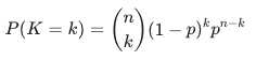
This formula is the precise theoretical description of the curve that was superimposed on the simulation’s histogram.
Pascal’s triangle is the geometric and recursive representation of the binomial coefficients. Its relevance to the random walk is profound:
- Enumeration of Paths: The
n-th row of the triangle lists the exact number of distinct paths that exist to reach each possible state in a symmetric random walk (wherep=0.5). Each entry in the triangle can be viewed as the number of possible “histories” or trajectories leading to that point. - Recursive Relationship: The construction rule of the triangle

has a direct physical interpretation: the number of ways to arrive at position(n,k) is the sum of the number of ways to have arrived at the only two possible preceding positions, namely ((n−1,k−1) and (n−1,k). The server simulation, even if asymmetric (p≠0.5), shares this same path topology.
If combinatorics provides the “counting,” then algebra provides the “structure.” The Binomial Theorem states that:

This theorem is the algebraic foundation of the binomial distribution. By substituting x=(1−p) (the probability of success) and y=p (the probability of failure), we obtain: ((1−p)+p)^n=1^n=1
This simple identity has a profound meaning: the sum of the probabilities of all possible outcomes (from k=0 to k=n successes) is exactly 1. The binomial expansion thus ensures that the terms P(K=k) form a complete and coherent probability distribution.
A more subtle but equally elegant connection exists with the Fibonacci sequence. While not directly apparent in the standard random walk, it emerges from a shared combinatorial structure.
- Sum of Pascal’s Diagonals: The Fibonacci numbers can be generated by summing the binomial coefficients along the “shallow” diagonals of Pascal’s triangle.
- Common Combinatorial Origins: This relationship is not a coincidence. Both constructs (binomial coefficients and Fibonacci numbers) are solutions to recursive counting problems. For instance, the Fibonacci number
Fn+1counts the number of ways to tile a1×npath with blocks of length 1 and 2. This “path-counting” with steps of varying sizes is a variation on the random walk problem. The connection reveals that the binomial random walk is a member of a vast family of combinatorial processes whose properties are deeply intertwined.
Conclusion
The server security simulation, while a practical computational model, serves as an empirical validation of fundamental mathematical theorems. This analysis has demonstrated that although the Bernoulli process is the common starting point, the analytical objective sharply distinguishes a random walk analysis (focused on the distribution of the sum) from that of the Law of Large Numbers (focused on the convergence of the mean).
Furthermore, the system’s behavior is entirely described by an elegant interplay of combinatorics (binomial coefficients as path-counters), algebra (the binomial expansion as a guarantee of a coherent distribution), and recursive structures (Pascal’s triangle). Understanding these connections allows one to move from a simple observation of simulation results to a profound comprehension of the mathematical principles that govern stochastic systems.